Journeyman’s Tips on Optimizing SQL Queries

Introduction

How you query your database matters. Sloppy queries can bring your website to a halt. Effective queries can make your data analytic platform run fast.

This article shares tips I use to make database queries work better. I don’t know all the tricks out there. We will explore those that actually helped me solve problems in live applications. For now, we will cover only tabular databases that support SQL–the most common group. Moreover, we will focus on techniques that don’t change the database structure.

If you want to run the examples yourself, go to this repository and follow its README.

SQL support and tabular vs. relational

We narrowed down the focus of this post to ‘tabular databases that support SQL’. Such definition may sound cagey, so let’s unpack it.

Tabular databases organize data into tables. By SQL support, we mean that we can use the structured query language to query them. This description fits a broad range of databases. It will allow us to cover many techniques that work for most of them without getting into details of specific databases.

We won’t need our databases to support the full SQL standard. Otherwise, we would end up philosophizing if any full ANSI-compliant database exists. We will generally work with a subset of SQL that most SQL-like databases support. When we use any features of a specific database, we will mention it.

Tabular database is not the same thing as a relational database. For example, Snowflake is tabular, but it won’t let you define relational constraints. You can create relations among datapoints even in non-relational databases. Yet only relational databases will enforce them for you. E.g., they will not let you delete a user without deleting their posts.

Databases for analytics tend to use SQL and be tabular but not relational. Several modern databases support a subset of SQL syntax and are not tabular. Here are some examples of major databases and their properties:

database	uses relations constraints	uses SQL	is tabular
PostgreSQL	✅	✅	✅
Snowflake	❌	✅	✅
CosmosDB	❌	✅	❌
MongoDB	❌	❌	❌

You probably noticed that we haven’t included every possible combination. For example, EdgeDB is relational, does not support SQL queries, and it is not tabular, even though it uses tables as an underlying storage. Dataphor, on the other hand, is both tabular and relational but lacks SQL support too.

Most databases I’ve come across fit into one of the categories listed in the table above.

Premature optimization

We hinted that you should optimize your queries to improve your applications’ performance. But not always. Is it a problem that a query takes ten minutes? What if it runs once a day, does not block any other queries, and processes terabytes of data? Maybe not a problem. What if it needs a huge Snowflake cluster, and the ten minutes cost you a ton of money. Well, then it might be a problem. But a query that takes 200 millisecond is surely not a problem, right? What if your application needs to run it a hundred times per second. Well…

Before you start optimizing, know the metric you need to improve. It can be cluster cost, database load, a response time of an endpoint, duration of some job, and many other things. Only then, you can actually decide how to optimize.

Only then can you decide how to optimize. Sometimes, the time you spend optimizing may outweigh potential savings. Other times, a larger database will give you the performance boost more cheaply.

Occasionally, fine-tuning SQL queries is your best bet. And that is the fun part that we will deal with in the rest of this article.

Our toy dataset

Throughout this article, we will be using a toy dataset with data for a fictitious website. We have tables of users, posts, comments, and visits. The data are pseudo-randomly generated ( see this repository). Although the tables are modest in size, they’re sufficiently large to show most techniques we’ll cover.

Horses for courses (OLAP vs. OLTP)

Are you working with the right type of database? You can copy-paste most of your Postgres queries and run them in Snowflake. Yet, these databases are useful for different purposes. Postgres optimizes for fetching individual rows quickly. Snowflake shows its strength on large data aggregations. On the flipside, you shouldn’t build a data lake on Postgres. And you should definitely avoid using Snowflake for low-latency applications.

I used to joke that every query takes a couple of seconds in Snowflake. No matter whether you are retrieving one row or aggregating millions of rows. Of course, it works up to a point, once you get to really large table, even Snowflake queries take minutes or hours. Postgres belongs to a family of online transactional processing (OLTP) databases. Snowflake, on the other hand, is an online analytics processing (OLAP) database.

Use OLTP if you need low latency, and OLAP if you need heavy aggregations.

A typical OLTP query might look something like this:

select email
from "user"
where id = 333
;

While an OLAP query might look more like this:

select u.name,
       substr(p.time_created::text, 1, 4) as year,
       round(avg(length(p.content)), 2)   as avg_post_characters
from "post" p
    inner join "user" u
on u.id = p.user_id
group by 1, 2
order by 1, 2
;

In real applications, both OLAP and OLTP queries can get a lot more complex than these examples. But let’s not get ahead of ourselves.

Our examples will work with PostgresSQL (aka Postgres), as an OLTP representative. I am planning to add more database examples to the playground repository in the future. Currently, I am thinking of Apache Druid and Clickhouse to get some realistic OLAP examples.

Most techniques that we will cover are useful for both OLTP and OLAP. In some cases, we might notice that they work only on one type of database. This is, among other reasons, because OLAP databases try to be smarter. Since they don’t need to respond within milliseconds, they can take more time to optimize query execution. The benefit of this is that a poorly written query can perform well in OLAP. The negative is that fine-tuning such query might not always work, because the query optimizer can translate both version to the same plan.

If you want to know more about different database types, read Designing Data-Intensive Applications by Martin Kleppmann. It’s the best book I’ve encountered on databases and related topics.

Isn’t SQL declarative?

You might have heard that SQL is a declarative language–you tell the database what you want, and it figures out how to get it. We will see that how you write your queries impacts their performance. Some people argue that this means that SQL is not declarative. Others say that declarativity does not guarantee that the database will always choose the optimal solution. There is an interesting discussion about this on StackExchange. We won’t delve into its details here. Let’s rather show that query structure matters on examples.

Understand your data

Databases make assumptions about your data. Tons of smart people have spent years optimizing and testing databases to make sure that these assumptions work well in most situations. But you can still do better than them. While a database can guess that a join will produce something between 1 and 30 million rows, you might know that it will be exactly one million. Or you might know that a filter removes 99 % rows in a table, so you will force the database to execute it as soon as possible. Or you might know that a table includes duplicate join keys, so, you deduplicate it before joining.

Suppose we want to display the last five visits of our website:

select *
from visit
order by timestamp desc
    limit 5
;

This is a straightforward query. We order the visits by timestamp, and then select the first five. Since the dataset is small, it doesn’t even take that long (around 200 ms on my computer). Now, if we’re aware that our website is getting regular visitors, we can make an educated guess about when the last five visits happened. It can be the last 10 minutes, 1 day, or whatever seems reasonable.

Then, we don’t need to sort the whole table:

select *
from visit
where timestamp > '2022-10-10':: date
order by timestamp desc
    limit 5
;

This is about twice as fast and gets us the same result.

But we can be even smarter about it without making the above assumption. We know that ids in the visit table are sequential, so, why not just use them. The id column is a primary key, so, it is indexed.

select *
from visit
order by id desc limit 5
;

This is about 80 times faster than the previous version, and 160 times faster than the original one. This last query did not need to scan the whole table, but just its index. Scanning an index is almost always faster than scanning the whole table.

We will discuss indices and their OLAP counterparts in a later section.

What else is running on your database?

Imagine that you wrote a query that is pretty fast and seems to work well. But when you run it in production, it starts to take ages or hangs indefinitely. Why?

There is a fair chance that your query is not the only one running on the database. Other queries might be blocking it, or it might not have the same amount of resources available as in your test environment. Furthermore, your application can run the query several times in parallel. Try to emulate production scenario. If the query should run 50 times in parallel in production, run it 100 times in parallel to make sure that the database can handle it.

In postgres, you can list active queries with this command:

select *
from pg_stat_activity
where state = 'active'
;

This query is database-specific. You will need to read documentation to get its counterparts in other databases.

Use diagnostic tools, particularly visualizers

Databases usually have a way to display how they decided to execute your query, i.e. describe the query plan. Studying it can reveal what the bottlenecks are. When I am optimizing a query, it is usually a back and forth between checking the plan and tweaking the query.

Sometimes, a query plan will show you on what parts of the query you should focus, but on some occasions, you will see that the query plan is suboptimal given your data. For example if order of joins is such that most data is filtered out at the end. In the latter case, you might try to push query planner into picking a better plan (see the section on Hinting).

I think execution plan visualizers are the most useful optimization tool. While you might struggle to find bottlenecks in the plan description, you will often see them from the first look at its visualization. Some SaaS database providers embed visualizers to their service. For many databases, there are also free versions.

Let’s see this on a simple example query. We want to find out if people are more likely to comment on posts from posters with the same email domain as they have. (Spoiler alert: They shouldn’t since the data is pseudo-random).

explain
(analyse , buffers , verbose)
select split_part(u1.email, '@', 2) as poster_domain,
       split_part(u2.email, '@', 2) as commenter_domain,
       count(*)                     as cnt
from comment c
         inner join post p on c.post_id = p.id
         inner join "user" u1 on u1.id = p.user_id
         inner join "user" u2 on u2.id = c.user_id
group by 1, 2
order by 1, 2
;

This is the query plan output by Postgres:

The 'cost' is Postgres' estimate of how expensive it is to execute part of the query. The actual time shows how long it actually took. If there's a big difference between the two, the query planner is more likely to choose a suboptimal plan. Consult Postgres [documentation](https://www.postgresql.org/docs/current/sql-explain.html) for more details.

QUERY PLAN
Finalize GroupAggregate (cost=152758.07..280612.17 rows=1000000 width=72) (actual time=1053.968..1141.873 rows=9 loops=1)
Group Key: (split_part((u1.email)::text, ‘@’::text, 2)), (split_part((u2.email)::text, ‘@’::text, 2))
-> Gather Merge (cost=152758.07..259362.17 rows=833334 width=72) (actual time=1045.034..1141.836 rows=27 loops=1)
Workers Planned: 2
Workers Launched: 2
-> Partial GroupAggregate (cost=151758.05..162174.72 rows=416667 width=72) (actual time=902.608..979.276 rows=9 loops=3)
Group Key: (split_part((u1.email)::text, ‘@’::text, 2)), (split_part((u2.email)::text, ‘@’::text, 2))
-> Sort (cost=151758.05..152799.72 rows=416667 width=64) (actual time=886.347..940.587 rows=333273 loops=3)
Sort Key: (split_part((u1.email)::text, ‘@’::text, 2)), (split_part((u2.email)::text, ‘@’::text, 2))
Sort Method: external merge Disk: 10528kB
Worker 0: Sort Method: external merge Disk: 9752kB
Worker 1: Sort Method: external merge Disk: 13112kB
-> Hash Join (cost=55962.05..97199.23 rows=416667 width=64) (actual time=315.504..733.590 rows=333273 loops=3)
Hash Cond: (c.user_id = u2.id)
-> Hash Join (cost=55592.05..93651.68 rows=416667 width=26) (actual time=292.296..561.203 rows=333307 loops=3)
Hash Cond: (p.user_id = u1.id)
-> Parallel Hash Join (cost=55222.05..92187.46 rows=416667 width=8) (actual time=290.426..480.756 rows=333332 loops=3)
Hash Cond: (c.post_id = p.id)
-> Parallel Seq Scan on comment c (cost=0.00..30987.67 rows=416667 width=8) (actual time=0.049..80.839 rows=333333 loops=3)
-> Parallel Hash (cost=48385.13..48385.13 rows=416713 width=8) (actual time=139.630..139.631 rows=333333 loops=3)
Buckets: 262144 Batches: 8 Memory Usage: 6976kB
-> Parallel Seq Scan on post p (cost=0.00..48385.13 rows=416713 width=8) (actual time=0.045..65.557 rows=333333 loops=3)
-> Hash (cost=245.00..245.00 rows=10000 width=26) (actual time=1.820..1.821 rows=10000 loops=3)
Buckets: 16384 Batches: 1 Memory Usage: 717kB
-> Seq Scan on “user” u1 (cost=0.00..245.00 rows=10000 width=26) (actual time=0.012..0.760 rows=10000 loops=3)
-> Hash (cost=245.00..245.00 rows=10000 width=26) (actual time=23.122..23.122 rows=10000 loops=3)
Buckets: 16384 Batches: 1 Memory Usage: 717kB
-> Seq Scan on “user” u2 (cost=0.00..245.00 rows=10000 width=26) (actual time=16.984..21.829 rows=10000 loops=3)
Planning Time: 0.532 ms
JIT:
Functions: 93
Options: Inlining false, Optimization false, Expressions true, Deforming true
Timing: Generation 8.097 ms, Inlining 0.000 ms, Optimization 5.882 ms, Emission 44.183 ms, Total 58.162 ms
Execution Time: 1150.066 ms

Sure, this query is not complex, so, reading the query plan isn’t that complicated once you get used to it.

But let’s compare it to the visualization of the same thing:

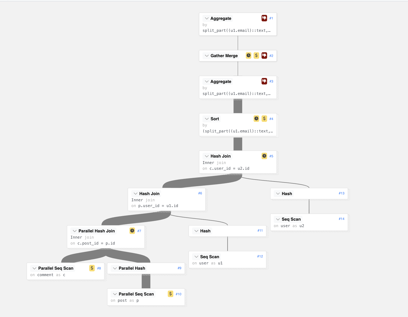
If you plug the textual plan into, e.g. Postgres Explain Visualizer, you get a nice output like the above.

Can you see how we could speed this query up? Suddenly, it becomes much clearer. We are not using indices, right? The graph shows several expensive operations that scan the whole table.

Clean up

A few years back, I had to speed up an application that computed several metrics for products. Users complained that it had gotten slower. I quickly realized that fetching data was the bottleneck–the actual computation took less than 5 % of the total endpoint response time. Strangely, there were tons of inactive products in the database, even though no one cared about their metrics.

When I deleted them, the critical endpoint got 3 times faster.

Deleting what you don’t need is one of the easiest ways to speed up your queries. If you do not have automatic cleanup processes in place, data tends to pile up. Since the queries need to run through more data, they get slower.

WHERE to strike

WHERE clause is often the first thing you should start playing with. The biggest improvements in query performance I have seen often came from changes to the filtering conditions.

Let’s look at an example query.

select u.name,
       count(*) / extract epoch
from (max(p.time_created) - min(p.time_created))) as posts_per_second_active
from post p
    inner join user u
on p.user_id = u.id
where lower (u.name) like '%helmut%'
  and p.time_created is not null
group by u.name
having max (p.time_created)
     > '2023-01-01'
   and max (p.time_created) != min (p.time_created)
order by time_per_post
    limit 10
;

SQL query engines evaluate query parts in the following logical order:

FROM and JOIN - determining the source data
WHERE - filtering
GROUP BY - splitting into groups
HAVING - filtering aggregated results
ORDER BY - sorting
LIMIT - limiting output rows

The actual order in which the SQL engine evaluates clauses may differ, but it must ensure that if you write your query as if it used the logical order, it will not fail or give inconsistent results because of that.

For example, we cannot get a zero division error in the query above even if the query engine decides to calculate posts_per_second_active before removing rows where max(p.time_created) = min(p.time_created).

In reality, the WHERE clause, or parts of it, might get executed even before tables are joined. The WHERE clause reduces the size of data we are working with from the start, and all next steps have easier job if they work with fewer data.

But a filtering clause that duplicates conditions already included in a join might actually slow queries down. Let’s compare these two queries:

Without an extra condition in the WHERE clause

select u.name,
       sum(c.upvotes_count) as total_upvotes
from "user" u
         inner join comment c on u.id = c.user_id
group by 1
having sum(c.upvotes_count) > 0
order by 2 desc limit 10
;

This takes about 218 ms on my machine.

Trying to add conditions to the WHERE clause or move conditions from the join there slows the query down. (Try commenting and uncommenting the WHERE clause or the HAVING clause in the query below to see the difference).

select u.name,
       sum(c.upvotes_count) as total_upvotes
from "user" u
         inner join comment c on u.id = c.user_id
where c.upvotes_count > 0
group by 1
having sum(c.upvotes_count) > 0
order by 2 desc limit 10
;

Both versions of this query (using only WHERE, or both WHERE and HAVING) take slightly above 300 ms on my machine.

We need a more complex query to benefit from putting logically unnecessary conditions to the WHERE clause.

Admittedly, the following example is a bit convoluted. Suppose we want to get a ranked list of users that visited our website in 30 days after a post was created. (They did not need to visit the post itself).

select p.id      as post_id,
       v.id      as visit_id,
       p.user_id as poster_id,
       v.user_id as visitor_id,
       u1.name   as poster_name,
       u2.name   as poster_name,
       row_number() over (partition by v.id order by v.timestamp) as rn
from post p
         inner join "visit" v on v.timestamp between p.time_created and p.time_created + interval '30 days'
    inner join "user" u1
on u1.id = p.user_id
    inner join "user" u2 on u2.id = v.user_id
where p.time_created
    > '2023-01-01'
  and v.timestamp
    > '2023-01-01'
;

As you can see, the v.timestamp > '2023-01-01' condition is not necessary. The inner join guarantees that v.timestamp >= p.time_created and p.time_created > '2023-01-01' is already in the WHERE clause.

Yet adding the v.timestamp > '2023-01-01' condition speeds up the query by about 40 % on my machine (500 ms vs. 300 ms).

Aggregation vs. sorting

Sorting is expensive. If you can, you should probably avoid it. I’ve seen quite a lot of code that sorts tables only to get a maximum of some column, i.e., where simple GROUP BY would suffice. Most often, such queries started out as more complex, and the sorting was originally necessary.

Let’s see this on an example. We want to get the id and the timestamp of the latest visit to our website:

select id, timestamp
from visit
order by timestamp desc
    limit 1
;

Later, someone decides that it is enough to return the latest timestamp, so, they remove the id from the query.

select timestamp
from visit
order by timestamp desc
    limit 1
;

What is wrong here? The query still sorts the whole table, even though we just need to compute the maximum of one column.

select max(timestamp) as timestamp
from visit
;

This does the same thing, is more memory efficient, and about 50 % faster on my computer. On a large table, the speed difference will be even more pronounced.

You will rarely see such a clear example in the real world. But, once you start looking for this pattern, you will spot it more often than you’d expect.

Subqueries

You should keep your queries as simple as possible. That will help both programmers and query planners. But sometimes you cannot express the business logic without nesting. Unless you decide to create a temporary table or view, subqueries and common table expressions (CTEs) are inevitable.

Occasionally, they can help you even if you can avoid them. For example, instead of cross joining tables and filtering the results, you may be better off de-duplicating them first. Then you join them without having to filter the result. Be careful though–the query planner might be smart enough to optimize the original (non-nested) query. Using subqueries can actually complicate its work.

Hence, this is something you have to test. There is no theoretical rule that will tell you whether using subquery is a good idea in particular case. What usually works for me is checking the size of the table in subquery before and after applying the subquery filter. If it is large and becomes much smaller after filtering, putting the filter into subquery might work. Otherwise, it usually won’t.

Let’s have a query that selects all posts that were updated in the 30 days after Alice Vaughan posted her post:

with temp_alice_post as (select *
                         from post p
                                  inner join "user" u on p.user_id = u.id
                         where u.name = 'Alice Vaughan')
select *
from temp_alice_post p1
         inner join "user" u on p1.user_id = u.id
         inner join post p2
                    on p2.time_updated between p1.time_created and p1.time_created + interval '30 days'
;

Filtering via CTE might seem like a good idea–we are reducing the post table to a small subset.

select *
from post p1
         inner join "user" u on p1.user_id = u.id
         inner join post p2
                    on p2.time_updated between p1.time_created and p1.time_created + interval '30 days'
where u.name = 'Alice Vaughan'
;

However, an experiment shows that the version without CTE is actually faster (630 vs. 350 ms on my computer).

Let’s try another example. We want to get names of people who visited our site more than 100 times. A straightforward query to do this would be:

select u.name
from "user" u
         inner join visit on u.id = visit.user_id
group by 1
having count(*) > 100
order by 1
;

But there is actually a faster way, despite being a bit uglier:

with temp_frequent_visitors as (select user_id
                                from visit
                                group by 1
                                having count(*) > 100)
select u.name
from "user" u
         inner join temp_frequent_visitors tfv on u.id = tfv.user_id
order by u.name
;

On my computer, the second query runs about 40 % faster (360 ms vs. 220 ms).

Use materialized views

I’ve seen countless examples of tables named like order_advanced, order_enriched, order_v2 order_extra. These boastful suffixes usually mean that the order_suffix table is the original order table with a few columns joined from another one.

I’ve also seen the horror in the eyes of hardcore programmers when they heard of such crimes against the laws of data modelling. The truth is that tables like these are common in analytical workflows, and, I daresay, even useful.

Imagine you have a team of ten analysts, each of them analyzing some aspect of sales. They all need data about orders and transportation costs, which is exactly what the order_advanced table provides. Of course, they could join the transportation costs themselves but that would slow their queries down. Moreover, they would need to duplicate the joining code creating a potential for mistakes. Sure, the data in this table will not reflect production at every moment. But if analysts don’t expect near real-time data, the partial inconsistency between production data and analytical datasets is not a problem.

Let us call tables that hold only data contained in other tables ‘derived tables’.

Another case where you might reach for such derived is an OLAP job. Instead of crafting complicated nested queries, you create temporary table simplifying query planner’s job, and delete them when job finishes.

A better alternative to a non-temporary derived table is a materialized view, which is basically a table that knows how to refresh its data. Materialized view is read-only. You can write only to underlying tables. On refresh, it runs the queries by which it was created. But making sure that the refresh happens when it should is a discipline of its own. (I will write another article on that).

Be aware of the difference between view and materialized view. Materialized view runs queries on refresh, and holds the data, i.e. it is a kind of ‘derived table’, whereas normal view runs its queries when you query it and does not hold any data.

Usually, using a materialized view is better than using persistent derived tables. Materialized view indicates that it is read-only. You can refresh it with one command, and you don’t have to send a long query to the server every time you want to do it. Then again, you might have good reasons to use derived tables, e.g., for compatibility with exporters to other systems or to make sure you store your code transparently somewhere else, and not in the database.

Apart from the column-adding transformations mentioned above, a good use-case for a materialized view might be something like this:

with temp_total_post_visits as (select post_id,
                                       count(*) as visits_count
                                from visit
                                group by 1),
     temp_recent_post_visits as (select post_id,
                                        count(*) as visits_count
                                 from visit
                                 where timestamp + interval '3 days' > (select max (timestamp) from visit)
group by 1
    )
select u.name,
       max(coalesce(trpv.visits_count / ttpv.visits_count, 0)) as recent_visits_share
from temp_total_post_visits ttpv
         inner join post p on ttpv.post_id = p.id
         inner join "user" u on p.user_id = u.id
         left join temp_recent_post_visits trpv on ttpv.post_id = trpv.post_id
where trpv.visits_count / ttpv.visits_count > 0.1
  and trpv.visits_count > 3
group by 1
order by 2 desc limit 100
;

This query creates a leaderboard of trending posters. We want to display it to our users on their home page. Recomputing all aggregations on every home page refresh would be too expensive. Instead, we can create a materialized view, and refresh it, e.g., once every ten minutes.

Indices, clustering keys, partitioning keys

If your query hits an index, you are in luck. Indices are the most common tool databases give you to speed up fetching or filtering records.

When your query hits an index, the database does not need to scan the whole table, and thus needs to read much fewer data. (This StackOverflow answer explains it well).

Indices work primarily in OLTP databases. If you can, you should directly compare against the index values in the WHERE clause or join and not use functions on the indexed columns. If you do, the database might not be able to use the index. This video provides a nice illustration.

Be careful when you read about indices in OLAP. Snowflake, for example, lets you define a primary key. You might think that it creates and index and enforces its uniqueness as a well-behaved database would. It doesn’t. Snowflake says in their documentation that they use constraints as a documentation feature. Creating a primary key in Snowflake does not even create an index. I am quite sure this has confused many people. Seeing duplicates in a primary key column certainly confused me.

In OLAP databases, you might encounter clustering, partitioning, or some other keys. These usually divide table into chunks. (We won’t go into too much detail here as partitioning and clustering techniques are database-specific).

If we take our post table from previous examples and set clustering key to the updated_at column, the database will ideally create chunks that cover mutually exclusive time intervals of updated_at . When your query hits a clustering or partitioning key, the database can skip all chunks that do not contain the key. If you do not hit the key, it needs to check all partitions.

If you decide to partition a table, you should choose a column that you often use to filter it. Often, databases will let you define only one partition column, e.g. BigQuery. In practice, people often partition by insertion date in append-only tables. This makes sense because if data grows in a reasonably similar pace in time, and you usually need to work with data for certain period.

Clustering keys, for example in Snowflake, are more flexible. You can define clustering key on multiple columns. BigQuery actually allows both partitioning and clustering. You can use any combination of the two methods.

Clustering or partitioning is primarily useful on larger tables (think > 1 TB). With smaller ones, the overhead of shuffling data might not be worth it. If you are paying for the time that database does something, as in Snowflake, you should also consider that clustering large table takes a lot of time and needs to happen regularly. Otherwise, the chunks won’t be balanced, and their benefits will fade.

Indices are the most flexible. You can usually define as many as you want. But bear in mind that each index takes up space and slows down writes to the corresponding table.

Let’s see how we can speed up a simple query by adding an index. Imagine we want to tally the posts created within a specific timeframe:

select count(*) as post_count
from post
where time_created between '2021-01-01' and '2021-12-31'
;

This takes about 100 ms on my computer. That might be great or terrible depending on the context. Let’s suppose it is too slow for our use-case, e.g., we need to run this query hundreds times per second and get the results quickly.

The time_created column is not indexed, so, the database needs to do a table scan. Let’s change that:

create index post_time_created_idx on post (time_created)
;

Now, we are at 10 ms, so 10 times speedup. The database needs to do index-only scan. Since we care only about the number of rows, it does not need to read any data from the table.

But even a query that needs to read some data, will be faster thanks to an index. Let’s count the number of unique posters in the same timeframe.

select count(distinct user_id) as posters_count
from post
where time_created between '2021-01-01' and '2021-12-31'
;

As in the previous query, we need to filter the table to the relevant timeframe. But here, we also have to read it and count distinct posters.

This takes about 100 ms without the index on time_created and about 40 ms with it.

I will not show examples with clustering or partitioning keys here. We would need to generate a lot more data to see their benefits. I’ll try to create such examples in the accompanying repository later.

Hinting

Hinting is a way to tell the query planner how to execute the query. You can do it either explicitly (e.g. via pg_hint_plan in Postgres), or by tweaking the query, so that the planner selects the optimal plan. I try to stay away from the first option. Unless the distribution of data is very stable, you can shoot yourself in the foot.

Explicit hinting interferes with query planner. It can lock you into a suboptimal execution plan, even if the planner could find a better one. Normally, Postgres’ cost-based optimizer estimates costs of different possible plans and selects the cheapest. If you use hints, you restrict its freedom of choice. There are situations when plan hinting is the best strategy, but, from my experience, they are rare. If you are not sure whether to use explicit plan hinting, don’t.

Sometimes, you might boost query performance by tweaks that make no apparent sense. Let’s see how I made a query almost two hundred times slower by removing an unnecessary join. (Regrettably, I couldn’t replicate this with our toy data, so I will use an actual example). The query extracts the first content block of articles published on the website:

select e2.id,
       mac.field_module_text,
       e3.handle
from matrixcontent_articlecontent mac
         inner join elements e on e.id = mac."elementId"
         inner join matrixblocks mb on e.id = mb."id"
         inner join entries e2 on mb."ownerId" = e2.id
         inner join entrytypes e3 on e2."typeId" = e3.id
where e."dateDeleted" is null
  and e.enabled
  and not e.archived
  and mb."sortOrder" = 1 -- the first article block
  and e2."postDate" is not null
;

This was a subquery in a larger query, but I will not copy the whole thing here as it would be hard to see the important parts.

While refactoring the code, I realized that the handle column is not used anywhere, so, I removed it. The output no longer included any data from the entrytypes table. You might think that the entrytypes table still filters something since I am using an inner join. But it does not, even though you cannot see it from the query alone: I am joining entrytypes on entries on entries.typeId = entrytypes.id. entries.typeId is a non-nullable column with a foreign key to entrytypes.id, and entrytypes.id is a primary key. Hence, if I remove the excessive join, the output will be identical.

That is what I did, hoping to see some performance improvement:

select e2.id,
       mac.field_module_text
from matrixcontent_articlecontent mac
         inner join elements e on e.id = mac."elementId"
         inner join matrixblocks mb on e.id = mb."id"
         inner join entries e2 on mb."ownerId" = e2.id
where e."dateDeleted" is null
  and e.enabled
  and not e.archived
  and mb."sortOrder" = 1 -- the first article block
  and e2."postDate" is not null
;

The execution time went from roughly 200 ms to more than 30 seconds, and I was not happy. When I kept the join there, the performance remained similar to the original. I took the subquery out and started looking into it, but then came another surprise. In isolation, the execution time did not worsen without the join. It turned out that when it was a part of a larger query, the join gave a hint to the query optimizer, and it chose a better plan.

So, I ended up with seemingly nonsensical query:

select e2.id,
       mac.field_module_text
from matrixcontent_articlecontent mac
         inner join elements e on e.id = mac."elementId"
         inner join matrixblocks mb on e.id = mb."id"
         inner join entries e2 on mb."ownerId" = e2.id
         inner join entrytypes e3 on e2."typeId" = e3.id -- does not filter anything, but hints query planner
where e."dateDeleted" is null
  and e.enabled
  and not e.archived
  and mb."sortOrder" = 1 -- the first article block
  and e2."postDate" is not null
;

The sad ending to this is that I was not able to discover the reason for the difference. When I tried to run Postgres’ analyze on the version without the unnecessary join, it just kept running forever.

The moral of this story is not that you should go crazy adding unnecessary joins to your queries, and hope that it will speed them up. But you should be careful when optimizing. Query planner can sometimes get hints from things that almost seem like a programmer’s mistake.

Validate in production

I might get burned at the stake for writing this: you have to test in production. Not only in production, not mainly in production, but testing only in a test environment won’t cut it. Not so long ago, I almost destroyed a production database by running a query that took 2 seconds to execute on my computer. It took around 7 seconds on test database. Both my computer, test and production were running the same version of Postgres.

Furthermore, the test database had the same data as production but was running on a bit weaker machine. It was only logical to assume that in production, the query would run for less than 7 seconds. Worst case scenario, it would take 30 seconds if there’s a lot of other queries running.

Wrong! It didn’t take 7 or 30 seconds. In fact, it failed to finish at all. The production database chose a different query plan, and almost committed suicide.

Even if test your query thoroughly in your test environment, you should not make too strong assumptions about its performance in production. You just have to try it.

Conclusion: Question and experiment

Most of the time, optimizing query performance is a rigorous proces. You rearrange clauses, trim off unnecessary data, choose the most efficient functions, measure changes, and repeat. We’ve covered a few tricks here, but there’s a lot more to explore. But sometimes, queries will be slow, no matter how much love and care you give them.

Then, you have to think more broadly. Can you get the data from somewhere else? Split the query into parts? Redefine the database structure? Do you actually need to return all data in this query? Who uses it? What for?

Always question your assumptions. Don’t feel foolish if you follow a hunch. Your instincts will sharpen over time. This is more of a general life advice. With that, we’ll wrap up the article.